Geometric Models

Geometric models are those that take a specific boundary (discontinuity), and deform/undulate it is no longer spherically symmetric with respect to the planet’s centre. The discontinuities you are most likely to undulate are probably the surface or seafloor, the Moho, and the CMB; though in principle you can create a boundary wherever you like and undulate it.

If you like, you can think of a geometric model as taking a 2D surface embedded within the Earth and moving it inward out outward radially, with the degree of stretching or shrinking depending on where on the globe you are.

As such, the geometric model files are not too complicated, as they consist of three coordinates: a series of latitude and longitude points (together forming a geometric grid), and a third variable defining the position of the boundary at each point on the grid. The third variable is either a depth or a radius (which you use depends on the boundary: radius may make more sense for the surface and depth for the Moho.

Crucially (and in both cases), the depth and radius are given with respect to the boundary’s depth or radius in the 1D case. Note that the undulations on a particular boundary are given as depth/radii with respect to the boundary in question itself. This means that an undulation of 1 km on either the Moho or the surface is given in your model file as +1000 at that particular point, not 6372000, 6372, or anything else. In the input files you set which interface this is in reference to, e.g., 6371 km km radius (or 0 km depth) for the surface. So if you are using PREM and have a Moho undulation dataset where the Moho’s point at each point on the sphere is expressed as a depth below the surface, you probably need to subtract 24.4 km from it, because that is the PREM Moho depth.

As an illustrative but pointless example, if you created a 3D geometric model file for the Earth’s surface but wanted the surface to be totally flat, you would have a series of latitude and longitude points (−90° to 90° and −180° to 180°) respectively, and the third variable would be an array of zeros (meaning no change in either direction from the surface position in the 1D case). If you were doing the same for the Moho, the array would be completely identical (all zeroes in the third variable) – it would be in the input file that you specify which boundary you are deforming.

Obviously the number of depth/radius points in your 3D model must match the number of latitude/longitude gridpoints you have. If you sample latitude and longitude each at a spacing of 1°, that gives you 180 × 360 gridpoints, each of which must have a value for the surface elevation or depth. You can choose the spacing that you want: 1° is probably fine for most things.

Creating new geometric models

The base structure for global scale, 3D geometric models is included in Ben’s AxiSEM3D GitHub repository. In short we have created two python files (etop01.py and moho.py) which can be used to create and edit topographic surface and moho geometric models.

*** TO DO: we should move it to the main one.

The python scripts available in the GitHub repository are able to write your Moho and topographic models to a format that will be read by AxiSEM3D. We assume some familiarity with python and that you are able to run the functions given and are aware of how they pass outputs to one another using return.

You are not obliged to use these scripts by any means, but they are designed such that the file structures, variable names, and sampling all match the template input files provided. If you have your own model which is in a similar gridded format and you want to convert it into something you can use, you should just be able to read in the filenames and use the same functions in the python scripts to write the output. It is always worth re-reading in a new model that you have created and then plotting it to make sure that it is doing what you think it is doing.

Crust 1.0 Moho:

• The Crust 1.0 Moho is sampled at 1° intervals and generally you will not need to resample this as the frequency changes. Certainly you cannot get to anything less than 1 ° resolution, as this is as good as the data gets!

• Some of the strongest gradients in Crust 1.0’s Moho are at the western edge of South America. Obviously this is not simply a coincidence - there is a good physical reason for it! Unfortunately, it does mean that the Moho and the seafloor/Earth’s surface end up being quite close to each other. This both shrinks elements (making timesteps small, and cost expensive), and risks the boundaries interpolating into each other (which stops the interfaces being conformal, and breaks the code).

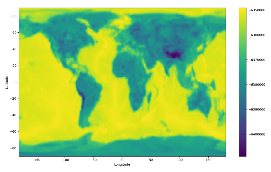
Crust 1.0 Moho undulation as a function of latitude and longitude. This plot shows the model with ° smoothing, sampled at 1°. For more details on the radial coordinates used, see below. Note that even with 1° smoothing, there are still strong gradients in Moho depth off the west coast of South America. We suspect that this area (or somewhere like it elsewhere in the world) is the cause of many issues.

ETOP01:

• ETOP01 is a global topographic/bathymetric model that is sampled at 1-arcminute resolution.

• 1 minute sampling is very much overkill for most projects, and is not feasible due to the amount of memory to store a model of this size. It should be downsampled to something more like 1 degree. If you want a more accurate determinant of how to downsample it, you can calculate the minimum resolved seismic wavelength at a particular period, and use a sampling which is at least as fine as this. Remember that as the period of the simulations you are running decreases (i.e., as the frequency increases), the waves become sensitive to smaller and smaller spatial structures, so you can get away with less downsampling.

• The strongest gradients in ETOP01 (by quite some margin) are also off the west coast of South America, where the Andes meet the coast and the subduction trench. We’ll come back to the errors that this can cause later, but you can get around some of it by applying some smoothing.

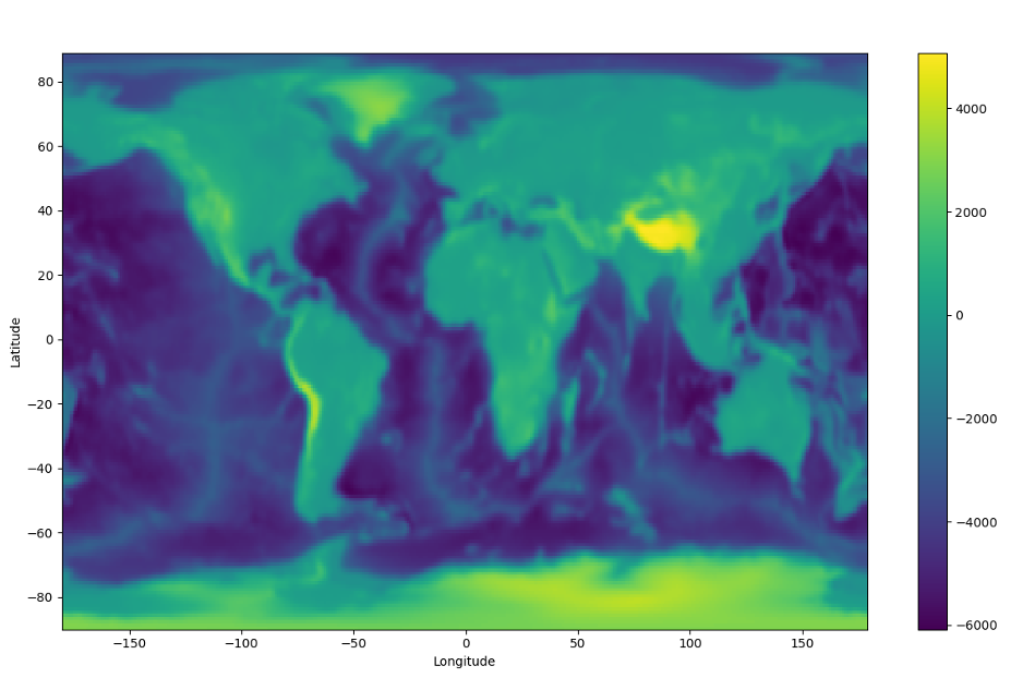
ETOP01, sampled at 1° and smoothed using a 1° sigma Gaussian. Again, note that the strongest gradients in topography are at the same locations as the strongest gradients in Moho undulation, i.e. at the western edge of South America.

Crust 1.0 Moho

Let us start with the Crust 1.0 Moho script because it is somewhat simpler to understand. The script is called moho.py and takes as input a grid file (.xyz) called depthtomoho.xyz which is a list of latitudes, longitudes, and moho depths at each pair therein.

The first function,load_moho_dat, takes the input file and uses a series of numpy functions to split it, for simplicity we have only actually kept the 3rd column ([2] in python) which is the depths, and re-created the latitude and longitude from scratch. Make sure that the coordinates are sorted in ascending order (-90° to 90°, -180° to 180°) or else the code will not like it.

The second function, write_data_to_netcdf_file, writes the inputs of the above function to a netcdf file. If you have not come across netcdf files before it is worth looking them up, they are basically a highly efficient way of storing data. Unlike ASCII files you don’t need to worry about pairing up the points correctly, within each file is a header called latitude (similarly for the other variables) which contains the points you have created.

There are a few stages to writing your new model file into netcdf format. First you need to create the file using Dataset (a method in the python netcdf4 module), and then create the three dimensions. You can specify the length of each dimension (latitude being 180 points, longitude being 360), or set this to 0 to allow them to grow as needed.

Then, you need to create the variable spaces to go with the dimensions you have created, and specify that the values will be floating point numbers (d). Finally, you add the actual points into the variable fields. Make sure that the units match, add corrections for metres to kilometres or vice versa if needed.

Note that if at any point you get errors about not being able to open a file, that is probably because it is already open. You just need to close it before opening it again.

Finally, read_data_from_netcdf_file allows you to just reload, and if you want to, plot (set plot=True) the saved netcdf file to check that it looks like what you think it should look like.

ETOP01

Using the ETOP01 script is slightly more complicated than using the Moho one, because you need to downsample (and possibly also average or smooth) the topography from the raw file that you download for the reasons that we already discussed.

The functions in etop01.py are similar to those in moho.py but with a few of additions. When you read in the raw model, there are two things that you can do to it:

• Average: average across n datapoints to produce a new topographic model.

• Filter: smooth the gradients in the new topographic model out using a gaussian filter.

If this seems confusing, consider that average basically means that you take a set of n by n points in the original 1-arcminute resolution model and represent their average as a single point in your new topographic model that AxiSEM3D is going to use. Choosing how big n is allows you to choose how fine your new model is (larger n = coarser model because a larger area is being represented by a single new elevation point). Once you have your new model you can further smooth the gradients in it by applying a 2D filter (like a blurring filter on Instagram).

The default sampling that we have chosen for the new 3D model is 1°, to match what is used for the Moho. If you want to change this it is relatively straightforward, just edit the relevant functions in etop01.py.

Rather than just simply choosing the midpoint of every 1×1° cell you instead take the arithmetic mean of each 1×1 arcminute cell within it to create your new elevation point (method 1). This naturally averages out extremes in your new model, and makes it less likely that the Jacobian will be badly behaved. We can get this to work for around 10s period global runs, but not 5s. This is probably because some of the gradients are still too large to be stably interpolated by AxiSEM3D. The issue is likely off the coast of South America, where a trench and an altiplano are found in close proximity. If you are doing regional-scale runs away from this area that might solve the issue, but in the more general case, you need to use a filter (method 2).

Starting with method – an average across each 1×1° degree cell – the copy of ETOP01 provided in these files is then filtered using method 1 a 2D 1° degree standard deviation Gaussian In effect, this treats the output array from the averaging as an image and applies a slight blurring filter; or technically a 2D convolution with a Gaussian kernel.

This simply smooths out some of the largest gradients in averaged array. You can choose how much smoothing happens by changing the value of sigma in filter_data. The default is 1°, reducing this toward zero makes the Gaussian kernel steeper and narrower and reduces the degree of blurring (in the limit of a zero standard deviation, the original image is returned). Similarly if you still get an error, you can increase the standard deviation which smooths out even more of the gradients. Note that you do not need to pass the units of sigma to the code, it does this in terms of sampling points (i.e., 1 ends up being 1  because there are 180 × 360 points, i.e. one per degree). If you do edit the python script to change the sampling, make sure the units of sigma are also changed to match.

Note that there are potentially some issues associated with switching from grid-centred to cell-centred systems at the poles – see the moho.py file for some comments on this topic.

Note on Efficiency.
Two aspects go into optimising a geometric model for efficiency:

1. The smaller the undulation range is, the smaller the “squashed” elements inside the undulation range become. This lowers the required time-step for undulated region in equal measure. And, unless there is a part of the medium requiring even smaller time steps, this makes the run more expensive.

2. When using ACA optimisation (see section on Nr field), undulated ranges require higher azimuthal resolution. So, from an ACA perspective, it would be ideal to keep the ranges as small as possible.

For most 3D geometric models there is hence an optimally efficient size for the undulation range. It is by no means necessary to find this exact range to perform an efficient simulation, but it is worth keeping in mind that there are two competing effects at play.