Plotting Seismograms

Once you have created a Trace object, plotting the seismogram is trivial. You can either use the built-in method that Trace objects have, but we prefer to use matplotlib.pyplot as you get much more functionality and user-control.

To do this, inside the plt.plot command you just reference the Trace’s time points and data points separately, using trace.times() and trace.data. Note that the data points are not called (i.e., no parentheses) but the time points are.

You can edit the figures using the same functionality you would for any other matplotlib plot, for example by setting labels, axes, linestyles, etc. You can also write relatively simple routines for doing things like plotting record sections (codes not included for simplicity – email us if you want them).

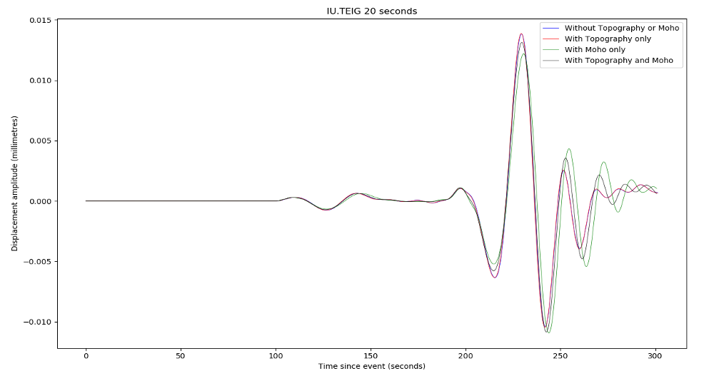Example seismograms. Note that the Moho undulations had to be smoothed to 10% of their original amplitude to make this run work, but some differences are still appreciable.

Filtering and convolution

If you used a delta function source, you need to either filter or convolve the Green’s function to return a result that is free of ‘noise’ at above the mesh frequency. It is worth thinking about the subtle differences between ObsPy’s filter routines and SciPy’s convolve ones.

In the broadest sense, these are of course identical, as filtering is equivalent to a multiplication with a kernel in the frequency domain, as is convolution. However, the way in which these are implemented can vary, and you also need to think about how convolution ends up being more complex in a numerical sense (with finite windows) than it is in the simplest, infinite-domain analytical sense.

Butterworth bandpass filters

The simplest kind of filter that you might want to use is a Butterworth-bandpass filter, whose functionality is included in ObsPy at obspy.signal.filter.bandpass This is as close to a ‘rectangular’ filter as you will want to get, for technical reasons simply removing all frequencies not between your two limits tends to give you numerical artefacts. A Butterworth-bandpass filter has steep, but not vertical sides. You can also choose the filter order (corners), and need to specify (default four) corner frequencies. In certain cases we have also found that running the filter both ways across the data (zerophase=True) can help.

For synthetic data, which effectively contain no noise other than that above the mesh period, the Butterworth-bandpass filter is a good choice. You can cut out the high-frequency noise by simply setting freqmax to the inverse of the mesh period, and you can remove low-frequency energy below 100 s by setting freqmin to 0.01. This is worth doing because, strictly speaking, frequencies below 100 s (i.e. 0.01 Hz) are not simulated properly in AxiSEM3D because we have no ellipticity, rotation, or gravity.

If you were using actual data, with a non-white noise content, another filter might be more appropriate: for example a log-gabor filter, which does not come installed in ObsPy (We can also send it to you though).

Convolution with a Gaussian function

Convolution with a Gaussian using SciPy ends up being a bit more challenging than you might think – on a qualitative level, it is just equivalent to swapping the frequency-domain representation of the Butterworth-bandpass filter for the frequency-domain representation of a Gaussian, which is also conveniently another Gaussian.

However, if you use scipy.signal.convolve, you need to make sure that the convolution parameters of the Gaussian (or indeed whatever other source-time function with appropriate frequency content you might wish to use) are set correctly. This includes matching the sampling rates (you can use ObsPy’s Lanczos interpolation to do this), and ensuring that the convolution mode is set to valid – to avoid padding out the seismogram with fake data points at either end.

Other operations and commutativity

In an analytical sense, all these operations should commute and it should not matter which order you do them in. In a numerical sense, this does not always appear to be the case (though this may just be due to poor processing on our part). So if something does not look right, try playing around with the order of operations.

We have also found that applying a taper to the seismograms can help, as if the end of a Green’s function trace includes a large non-zero displacement when the simulation ends, sometimes the convolution can produce a seismogram with an overall non-zero slope (i.e., trending to negative values over time), which is of course nonsensical.